RELION3.0 Tutorial

Try to use the frequently-used approach to cryo-EM structure determination
更新(2022.01.05)：
其实没想到当时自己摸索时的记录能给大家带来帮助，甚至还有以色列的朋友联系我，真的很开心，但是也真的很惭愧，早知道写得认真一些了，抱歉抱歉…….而且也很遗憾没能继续做电镜相关的内容了，也不好继续完善这个tutorial了，但电镜图像处理确实还是很有趣也很有意义的方向，而一开始也可能会走很多弯路而郁闷，如果大家对tutorial有一些问题，可以直接email我(wujg1995@163.com)，包括cryoSPARC，我也会一些，但是都不精而且没有继续用了，但如果我能帮忙解决的，是很愿意回复大家的；此外，之前有朋友问有没有PDF方便看，我传到百度网盘了，大家可以直接下载，如果有问题也可直接email我，链接：https://pan.baidu.com/s/1r0UpAviHOGvxnSdTGpyipw 提取码：hhhh
最后，祝大家科研顺利，子刊起步，搏一搏正刊！

1 预处理

1.1 建立项目

1、建议为每一个项目创建一个单独的路径，称之为项目路径，必须要在项目路径下打开RELION软件，之后所有操作都在该路径下

2、建立Movie文件夹放原始图像或者视频（MRC or TIFF）；如果不把原始数据放入Movie文件夹，需要创建符号链接，用于指向实际存放地址

3、如果我们下载了tutorial的测试数据，the (Movies/) directory was created. It should contain 24 movies in compressed TIFF format, a gain-reference file (gain.mrc) and a NOTES file with information about the experiment.

4、每次打开RELION都需在该项目路径下

relion

and answer “y” to set up a new relion project here.

5、将数据导入流水线，选择import job，然后填入参数：
• Input files: Movies/*.tiff
• Node type: 2D micrograph movies

导入完，可以在当前目录下输入以下指令查看导入的文件：

less Import/job001/movies.star

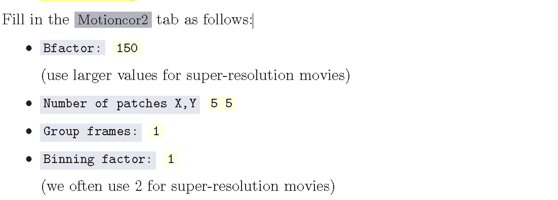
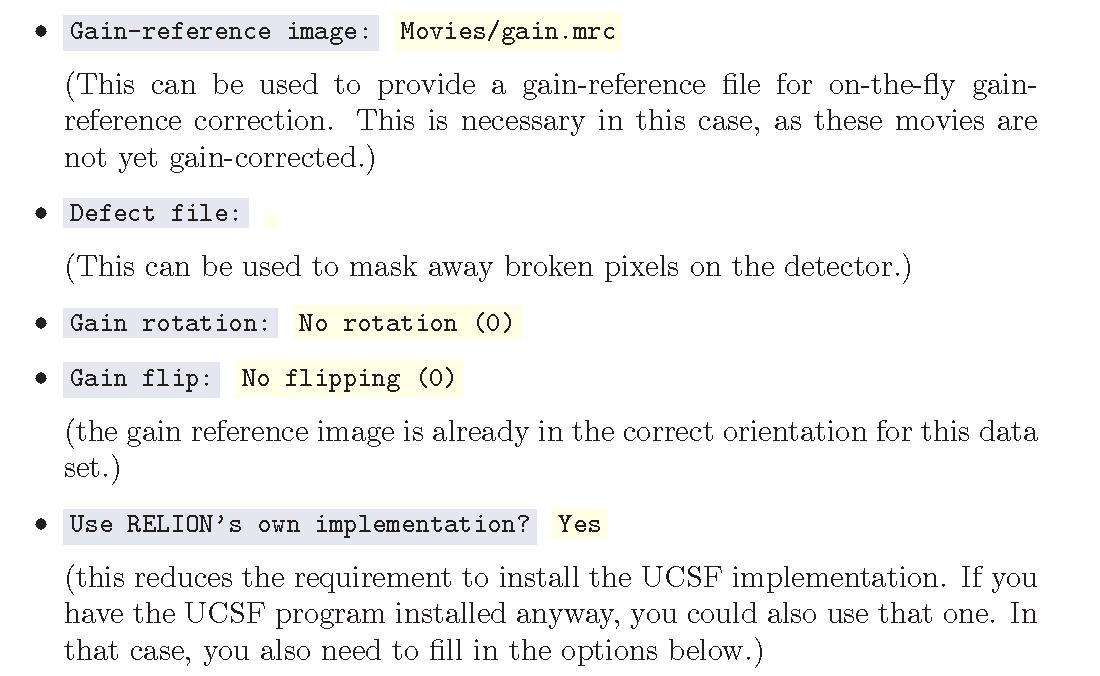
1.2 运动校正 （Beam-induced motion correlation）

由于电子光束穿过薄样品，会对样品产生损耗并使得其产生轻微位移，所以先需要对每张图像进行运动校正，使其图像的拍摄中心一致，参数设置:

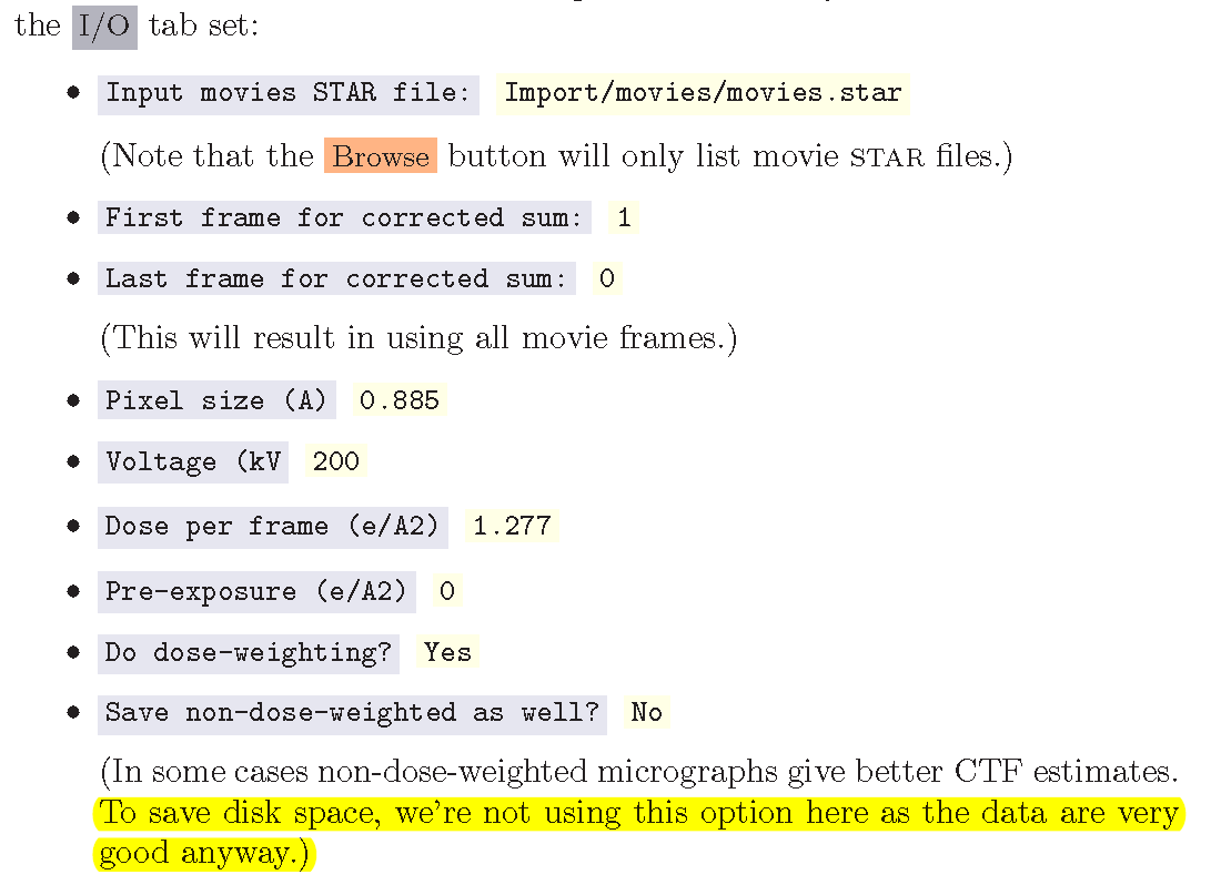
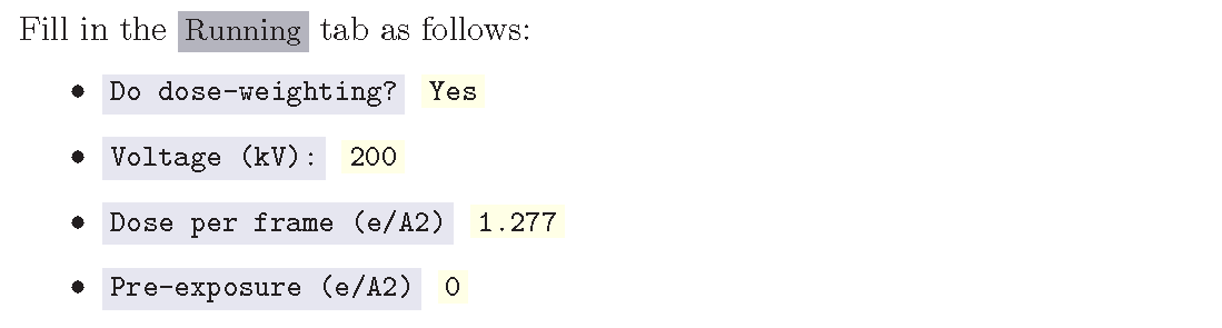
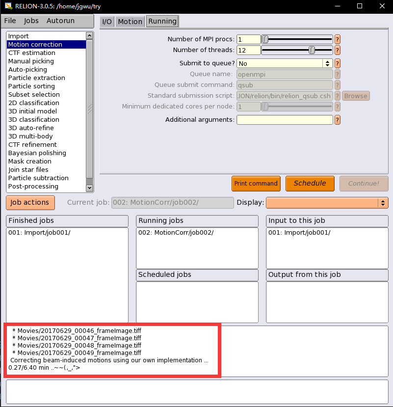
这个tutorial上的relion版本可能与我们节点上的relion3.0版本不一样，因为上述提到的Running的tabs里的参数都是I/O的tab里的字段，真正需要在running里填的字段就是:
Number of threads:12
(后面有解释，这个线程的数量最好能够被movie frames的数量整除，因为样例中有24个，所以选择了12，每个线程2个frame，则大约需要5分钟)

点击RUN，则看到下方的输出框开始输出当前步骤：

这个校正好了之后，我们可以通过点击选择Dispaly中的logfile.pdf，或者corrected_micrographs.star 查看加和完的micrograph，查看的具体操作如下：
You can look at the estimated beam-induced shifts, and their statistics over the entire data set, by selecting the out: logfile.pdf from the Display: button below the run buttons, or you can look at the summed micrographs by selecting out: corrected_micrographs.star.
为了使得corrected_micrographs能比较好的显示出来，需要调整显示的参数，具体操作如下：
设置参数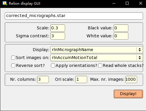

点击Display！，则显示出了颗粒的图像：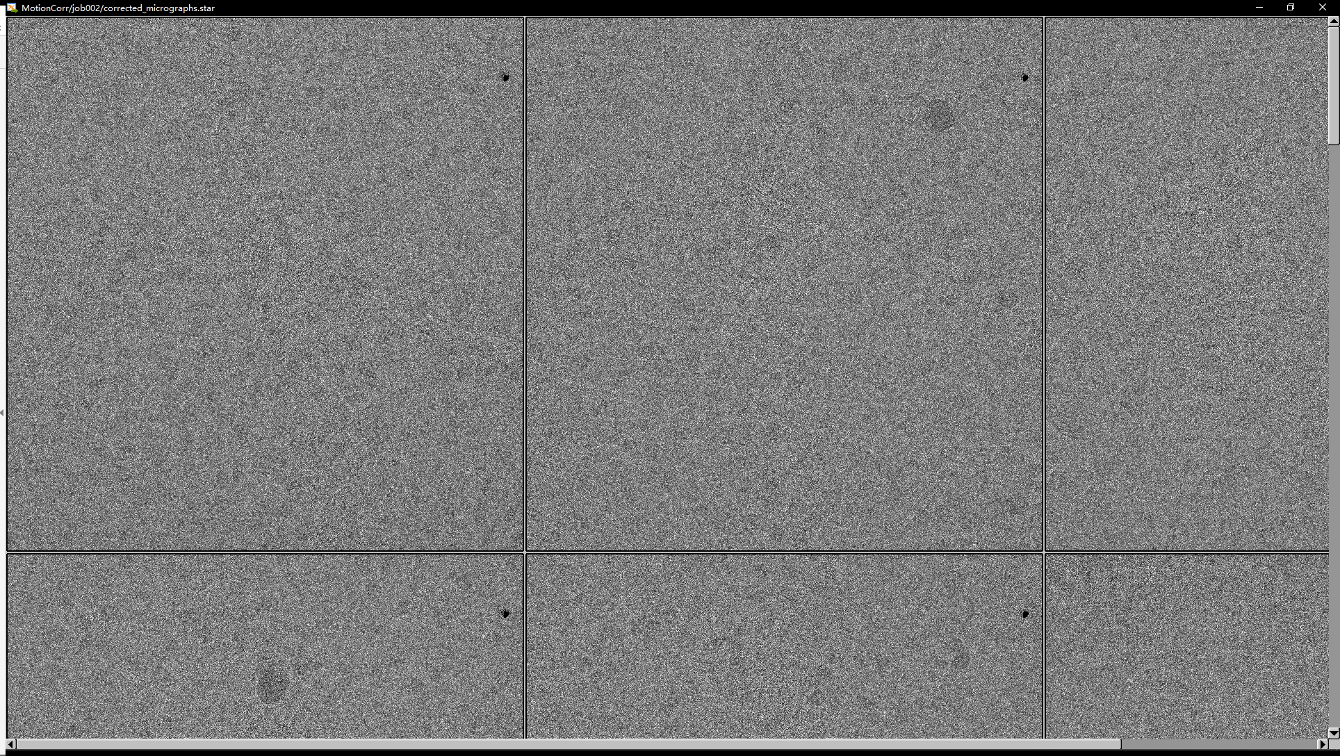

Depending on the size of your screen, you should probably downscale the micrographs (Scale: 0.3) and use Sigma contrast: 3 and few columns (something like Number of columns: 3) for convenient visualisation. Note that you cannot select any micrographs from this display. If you want to exclude micrographs at this point (which we will not do, because they are all fine), you could use the Subset selection job-type.

1.3 衬度转换函数估计（CTF estimation）

由于电镜本身的成像过程，会存在球差、离焦量等问题，需要对其进行分析，找出其CFT，对图像进行校正。这一步就是对于每个运动校正完的图像，预估比较合适的parameters，然后RELION这步有两个选择，张恺博士的GCTF或者没有GPU的话用Alexis Rohou and Niko Grigorieff’s ctffind4.1，接着开始填参数吧：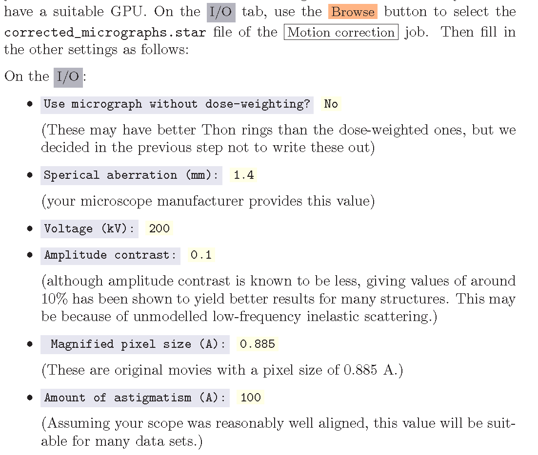

然后tutorial用的就是GCTF，所以searches和CTFFIND-4.1两个tab可以跳过，直接到GCTF设置：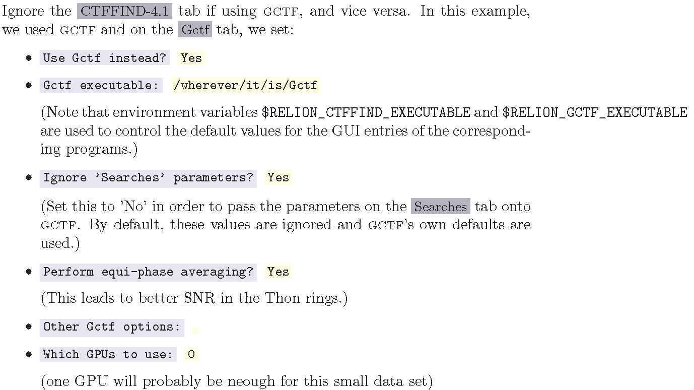

然后同样的Running部分，不需要其他的进程通信，1个就好，然后点击RUN
You can run the program using multiple MPI processes, depending on your machine. Using only a single processor and GPU, the job took 31 seconds with gctf. Once the job finishes there are additional files for each micrograph inside the output CtfFind/job003/Movies directory: the .ctf file contains an image in MRC format with the computed power spectrum and the fitted CTF model; the .log file contains the output from ctffind or gctf; (only in case of using ctffind, the .com file contains the script that was used to launch ctffind).
You can visualise all the Thon-ring images using the Display button, selecting out: micrographs_ctf.star. The zeros between the Thon rings in the experimental images should coincide with the ones in the model. Note that you can sort the display in order of defocus, maximum resolution, figure-of-merit,etc. The logfile.pdf file contains plots of useful parameters, such as defocus,astigmatism, estimated resolution, etc for all micrographs, and histograms of these values over the entire data set. Analysing these plots may be useful to spot problems in your data acquisition.If you see CTF models that are not a satisfactory fit to the experimental Thon rings, you can delete the .log files for those micrographs, select the CtfFind/job003 entry from the Finished jobs list, alter the parameters in the parameter-panel, and then re-run the job by clicking the Continue now button.Only those micrographs for which a .log file does not exist will be re-processed.You can do this until all CTF models are satisfactory. If this is not possible,or if you decide to discard micrographs because they have unsatisfactory Thon-rins, you can use the Subset selection job-type to do this.

需要格外注意的是：
在Running的tab，需要设置跑程序的环境，而这个在tutorial里是没有的，然后由于我们服务器节点在本地文件夹是没有cuda之类的GPU资源，所以需要提交到服务器节点上，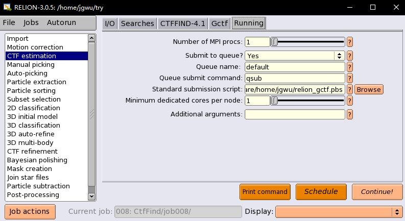
其中script是重点，需要编写脚本说明环境，
**

relion_gctf.pbs：**
#!/bin/bash
#
#PBS -l nodes=c002:ppn=2
#PBS -l walltime=120:00:00
#PBS -k oe
#PBS -q dx360k20
#PBS -N relion_ctf

cd $PBS_O_WORKDIR

#for c001~c009 nodes, queue dx360k20,x3650k40,default

module load cuda/8.0 intel/19.3 impi/19.3 tbb/19.3/gcc4.4 relion/3-cuda

#for amax/baode nodes, queue gpuw

#export PATH=/opt/openmpi-4.0.0/bin:/opt/relion-3/bin:$PATH
#export LD_LIBRARY_PATH=/opt/openmpi-4.0.0/lib:/opt/relion-3/lib:$LD_LIBRARY_PATH

#for avx acceleration

#module load intel/19.3 impi/19.3 mkl/19.3 tbb/19.3/gcc4.4 relion/3-avx
#export OMP_SCHEDULE="dynamic"
#export KMP_BLOCKTIME=0

mpirun XXXcommandXXX

其中，我们实验室节点上，前四个的显卡配置的是dx360k20，后面的是x3650k40 show

1.4 手动挑选颗粒（Manual particle picking）

这一步需要手动挑选颗粒在图像中的坐标，至少在多个几个图像中手动挑选，从而熟悉数据，并且手动挑选的将作为后面自动挑选颗粒的参考模板

tutorial中也说道，在3.0版本中，RELION提供了一个无参考的自动挑选（基于Laplacian-of-Gaussian (LoG) filter），而在目前大多数的测试情况中，这个方法都能提供比较合理的开始坐标，所以手动挑选这个步骤可以跳过，tutorial只对这个手动挑选说明一下，真正使用的是LoG的自动挑选生成颗粒的初始集合。

手动挑选颗粒非常依赖个人的专业经验，然后RELION也提供了很多挑选颗粒软件的接口，只要相应的文件保存好就行；

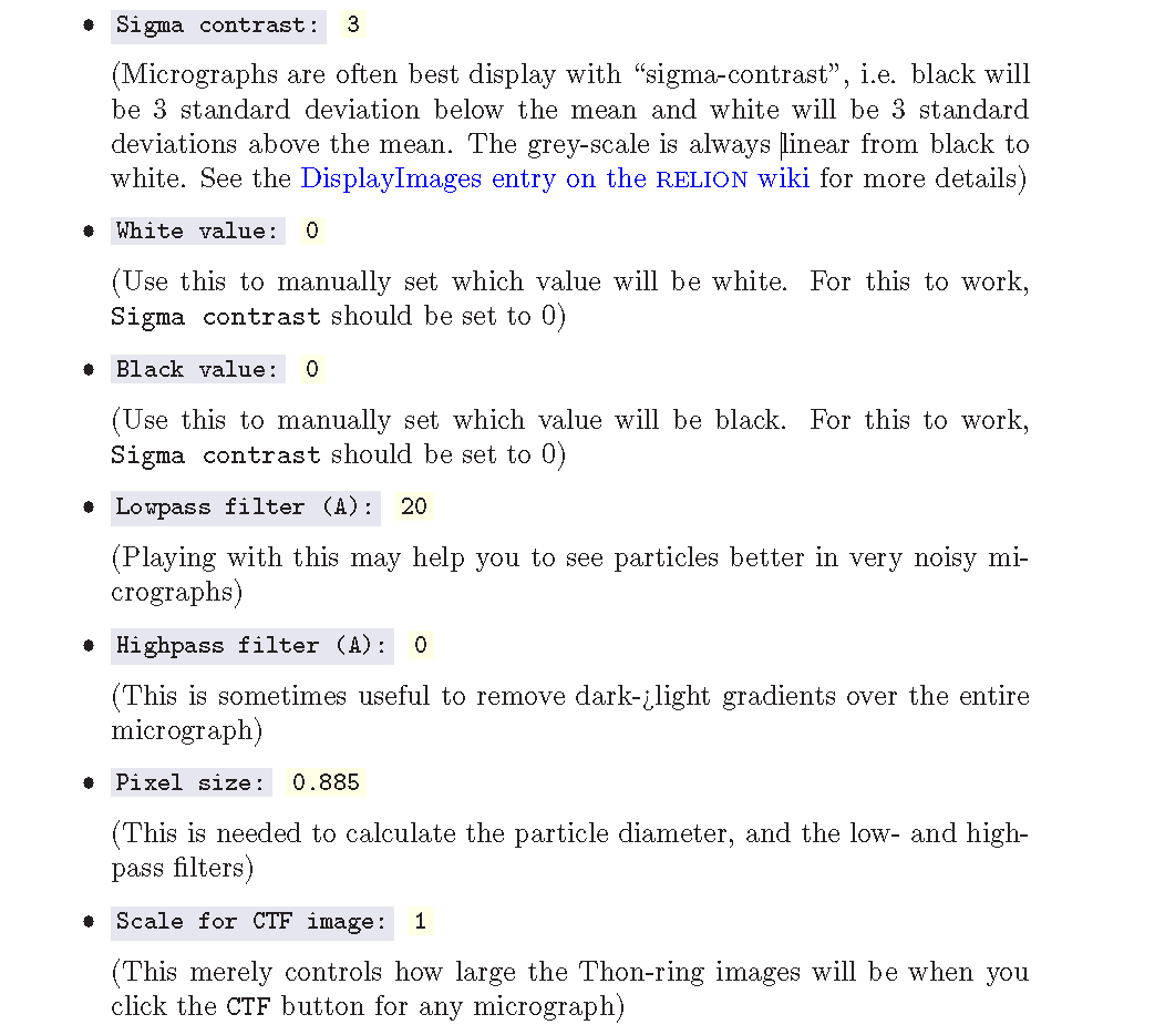
手动调训颗粒的参数设置：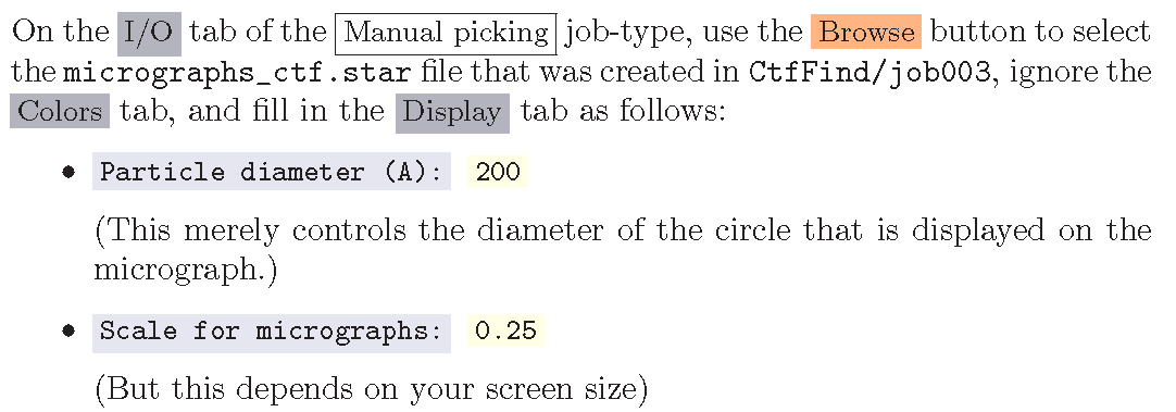

然后点击RUN，会出现：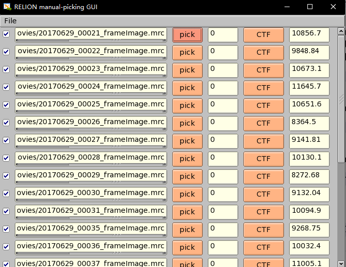

再点击pick，稍等会儿就出现：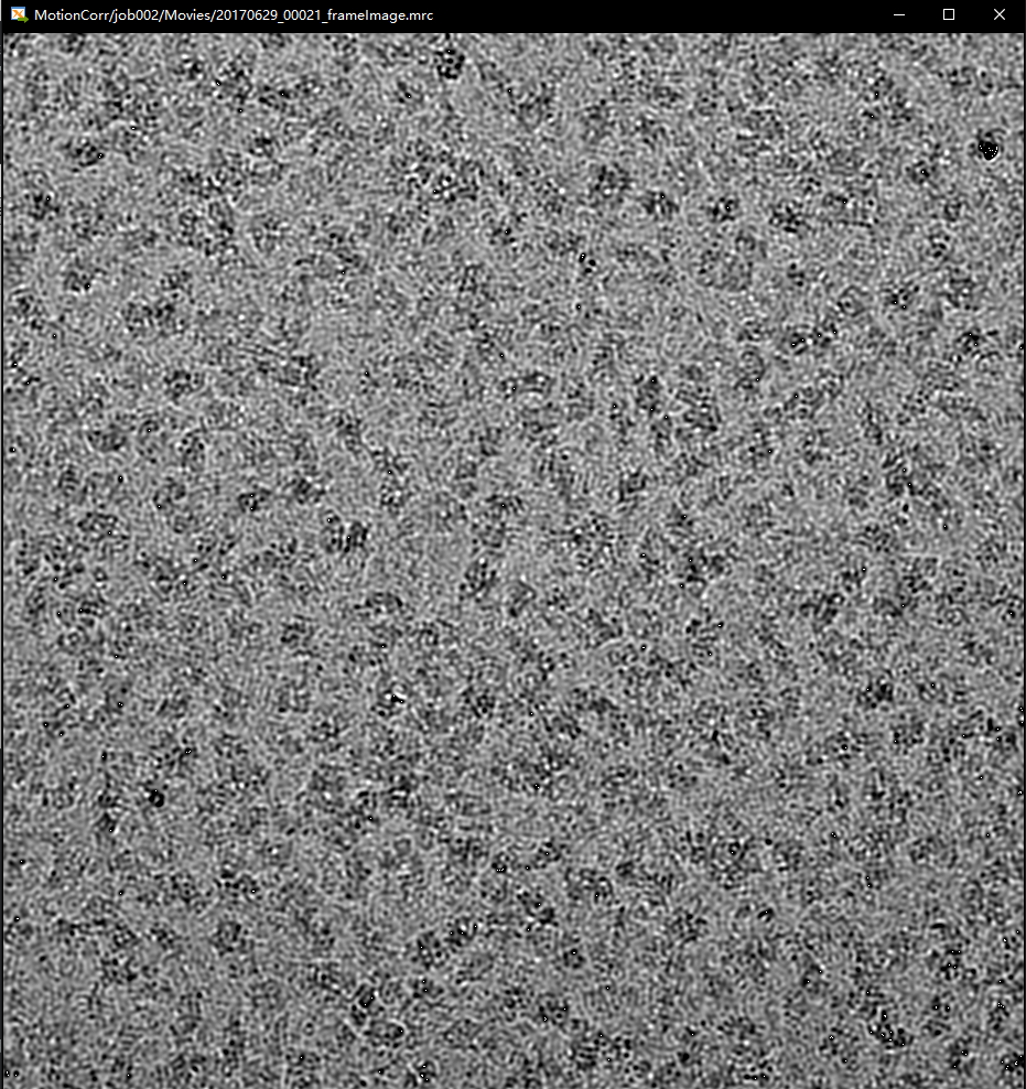

就可以挑选了，具体操作看英文就好，很详细：
Run the job by clicking the Run now! button and click on a few particles if you want to. However, as we will use the LoG-based autopicking in the next section,you do not need to pick any if you don’t want to. If you were going to use manually picked particles for an initial 2D classification job, then you would need approximately 500-1,000 particles in order to calculate reasonable class averages. Left-mouse click for picking, middle-mouse click for deleting a picked particle, right-mouse click for a pop-up menu in which you will need to save the coordinates!. Note that you can always come back to pick more from where you left it (provided you saved the star files with the coordinates throught the pop-up menu), by selecting ManualPick/job004 from the Finished jobs and clicking the Continue now button.

1.5 基于拉普拉斯-高斯算子的颗粒自动挑选（LoG-based auto-picking）

将通过这个办法挑选出颗粒的初始集，用于2D的classification去生成第二步自动挑选的模板；由于第一次不需要太多的颗粒，我们只在3张图像上使用该操作；

注意，一般情况下，可能会对所有可用的显微图执行基于LoG的选择，以获得尽可能好的模板。然而，在本教程中，我们只使用了一些显微图来加速计算。

先到 Subset selection 步骤，需要生成一个初始的图像集合用于自动挑选，具体操作看英文，很详细：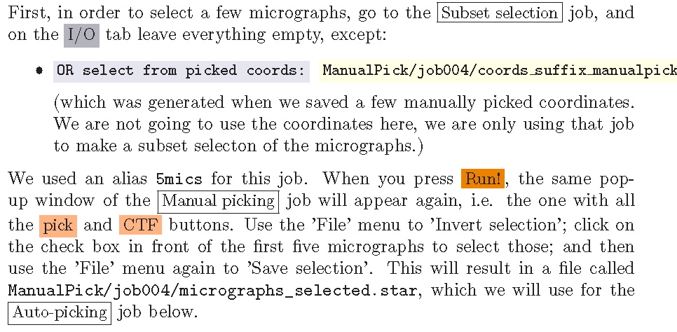

接着就可以开始Auto-picking了：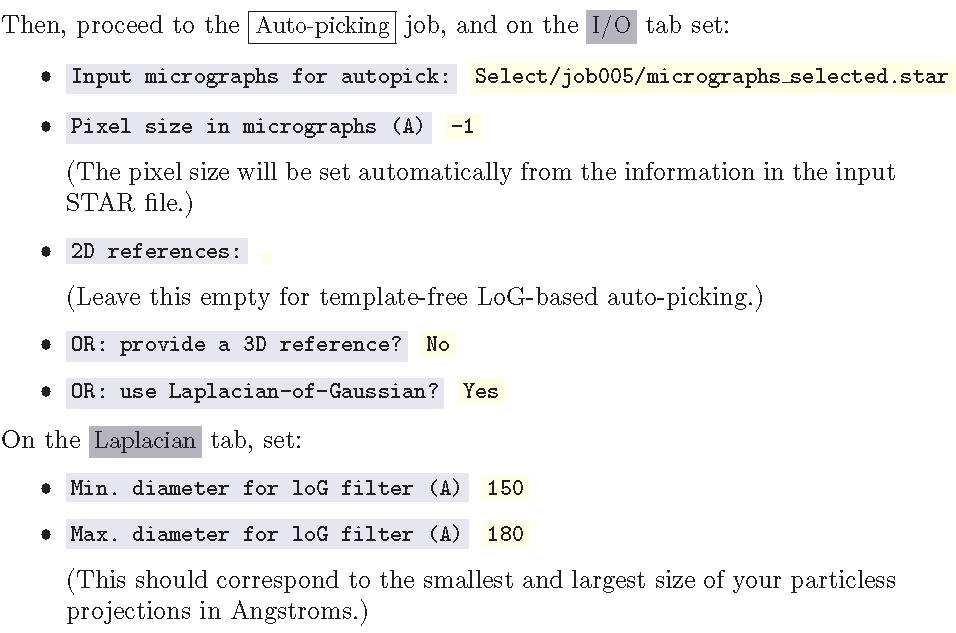

同样，需要提交队列计算，一会儿后就可以点击Display查看，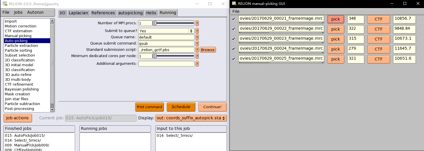
点击pick就可以看到已经自动挑选的颗粒：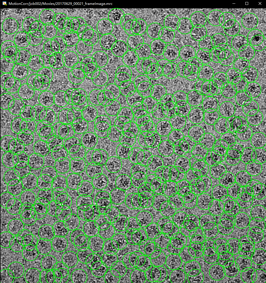

1.6 颗粒提取（particle extraction）

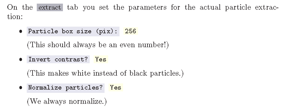
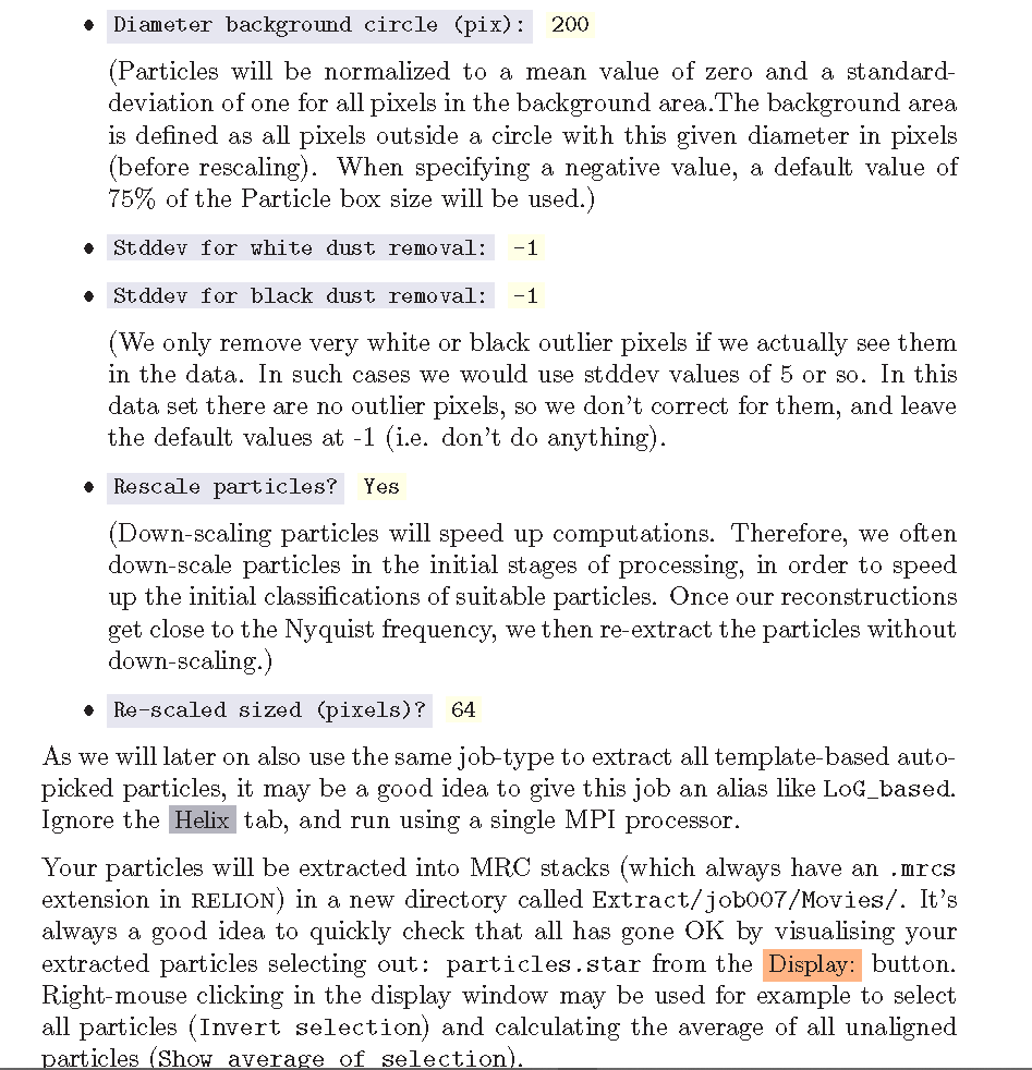
当每张想要挑选颗粒的图像都有了坐标文件后，我们就可以提取出对应的颗粒并收集到所有需要的元数据通过particle extraction：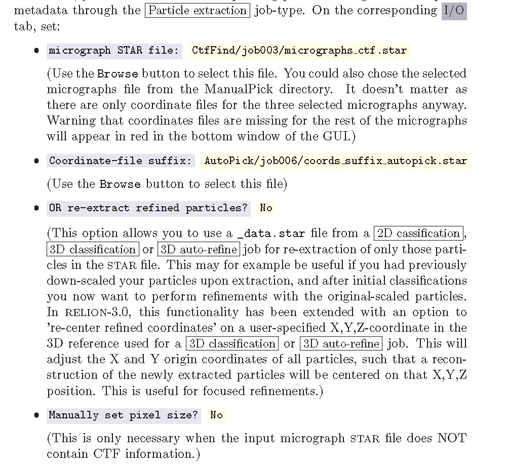

跑完之后，点击Display：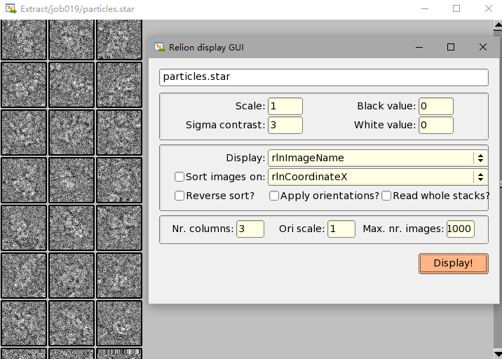

1.7 制作自动挑选的模板（Making templates for auto-picking）

为接下来对所有图像进行自动挑选计算出一个模板，我们将使用2D classification步骤：

现在I/O tab选中上一步extract出来的particles：
On the I/O tab, select the Extract/job007/particles.star
在继续在CTF tab 进行设置：
Do CTF-correction? Yes
(We will perform full phase+amplitude correction inside the Bayesian framework)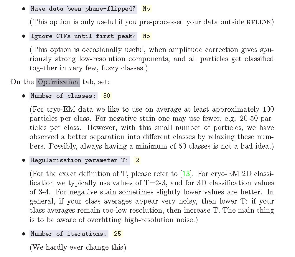





然后集群的话我看了下，c001-c005都只有两个gpu，c007-c009是1个gpu，amax01-02、baode01是4个gpu，我用的是c002，所以上面最后那个字段我填的是：0:1，
接着是下一页Running tab里的设置，同样的，我没根据tutorial里的MPI和threads的个数，我分别填了1和2，其他设置相同，queue name改成default，脚本也是之前那个，然后点击RUN，就提交到队列了，可以通过qstat查看任务状态，跑完后，通过Display查看：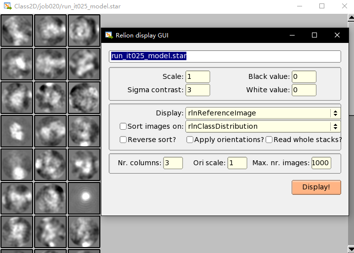

如上，显示出了50类颗粒的各自的模板
关于Running和Display：
On the Running tab, specify the ’Number of MPI processors’ and the ’Number of threads’ to use. The total number of requested CPUs, or cores, will be the product of the two values. Note that 2D classification , 3D classification ,3D initial model and 3D auto-refine use one MPI process as a master, which does not do any calculations itself, but sends jobs to the other MPI processors. Therefore, if one specifies 4 GPUs above, running with five MPI processes would be a good idea. Threads offer the advantage of more efficient RAM usage, whereas MPI parallelization scales better than threads. Often, for 3D classification and 3D auto-refine jobs you will probably want to use many threads in order to share the available RAM on each (multi-core) computing node. 2D classification is less memory-intensive, so you may not need so many threads. However, the points where communication between MPI processors (the bottle-neck in scalability there) becomes limiting in comparison with running more threads, is different on many different clusters, so you may need to
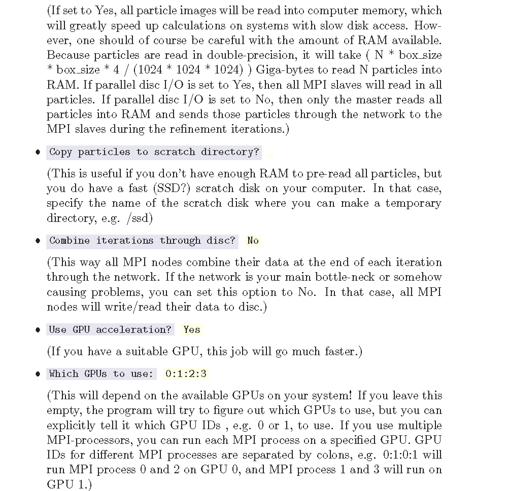
play with these parameters to get optimal performance for your setup. We pre-read all particles into RAM, used parallel disc I/O, 4 GPUs and 5 MPI process with 6 threads each, and our job finished in approximately four minutes.Because we will run more 2D classification jobs, it may again be a good idea to use a meaningful alias, for example LoG_based. You can look at the resulting class averages using the Display: button to select out: run_it025_model.star from. On the pop-up window, you may want to choose to look at the class averages in a specific order, e.g. based on rlnClassDistribution (in reverse order, i.e. from high-to-low instead of the default low-to-high) or on rlnAccuracyRotations.

1.8 选择自动挑选的模板（selecting templates for auto-picking）

在Subset selection中，选择合适的类平均图像；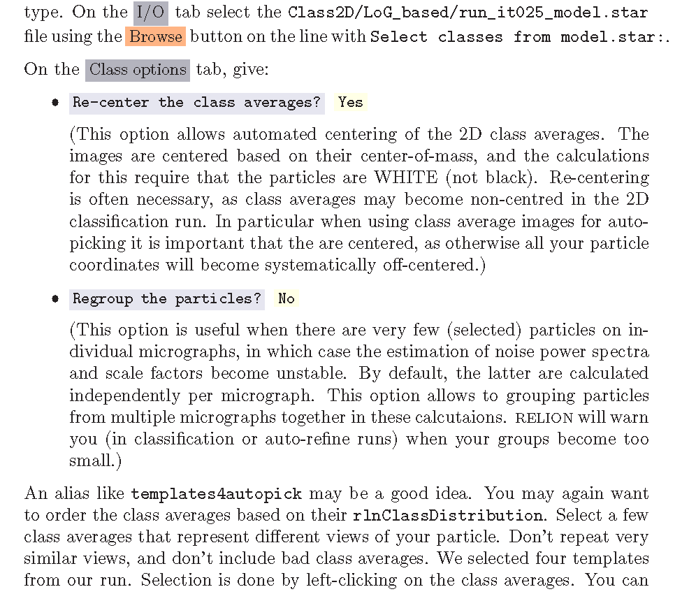

需要自己在Display中选择几个自己觉得是同一颗粒不同角度的类平均图像，不要找长得差不多的也不要找明显类平均完效果很差的，但是我也不知道怎么挑怎么好啊啊啊啊啊，随便左键点了几个凑合下，再右键save selected class保存

然后卧槽，最大的坑（may one of but now it is the worst ），一是不能随便选啊，这个非常关键啊，二是不是长得圆厉害啊，长得圆说明他模糊啊，那个圆是咱们的选中框啊，所以不规则的，明显的颗粒反而是好的，所以在class 2D查看的时候，勾上那个sort image 和 reverse，就是按类别的数量分布，然后选择前俩像饺子的那个（这是师兄教我先看了这个tutorial所用的颗粒的真实结构，然后看到有2D的图像，就选了这俩）：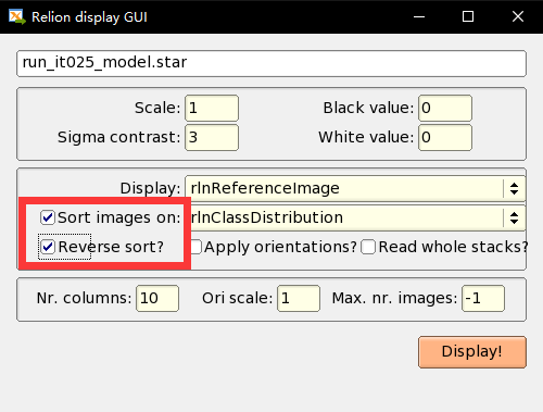

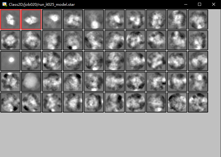
选择前俩，右键保存，完美！

真实的颗粒图像是：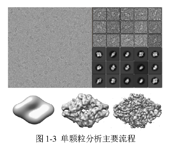

1.9 自动挑选(Auto-picking)

接下来，在通过视同选择的2D类平均作为模板，用于有参考的自动挑选

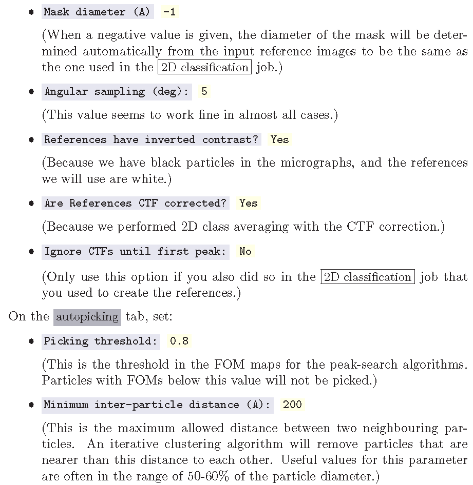
在所有图像上进行自动挑选前，我们需要优化Auto-picking步骤中autopicking中的4个主要参数：

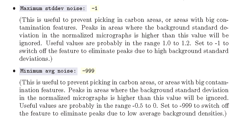
Picking threshold, the Minimum inter-particle distance,the Maximum stddev noise, and the Minimum avg noise.

为了节省时间，我们只在几张图片上进行操作；我们将使用之前LoG-based自动挑选出来的5张图片上；

最后一段提到的是，Auto picking的display窗口使用的参数是我们前面Manual picking中的，所以我们也可以在Manual picking job中修改参数，然后再relion界面的顶部jobs menu中选择save job settings，然后尝试了下修改Manual中clolor tab的参数：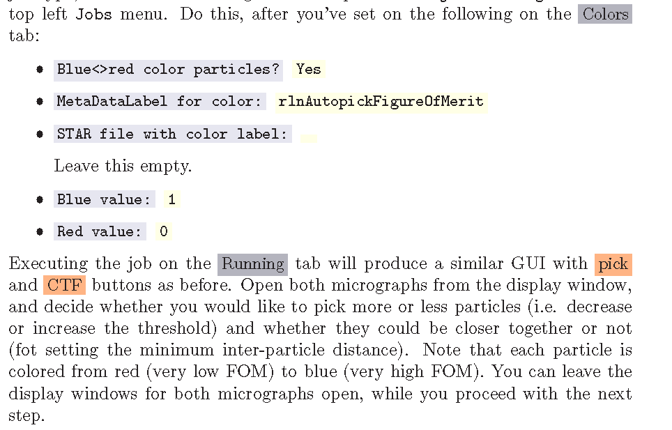

接着，选中AutoPick job,修改autopicking tab的参数：
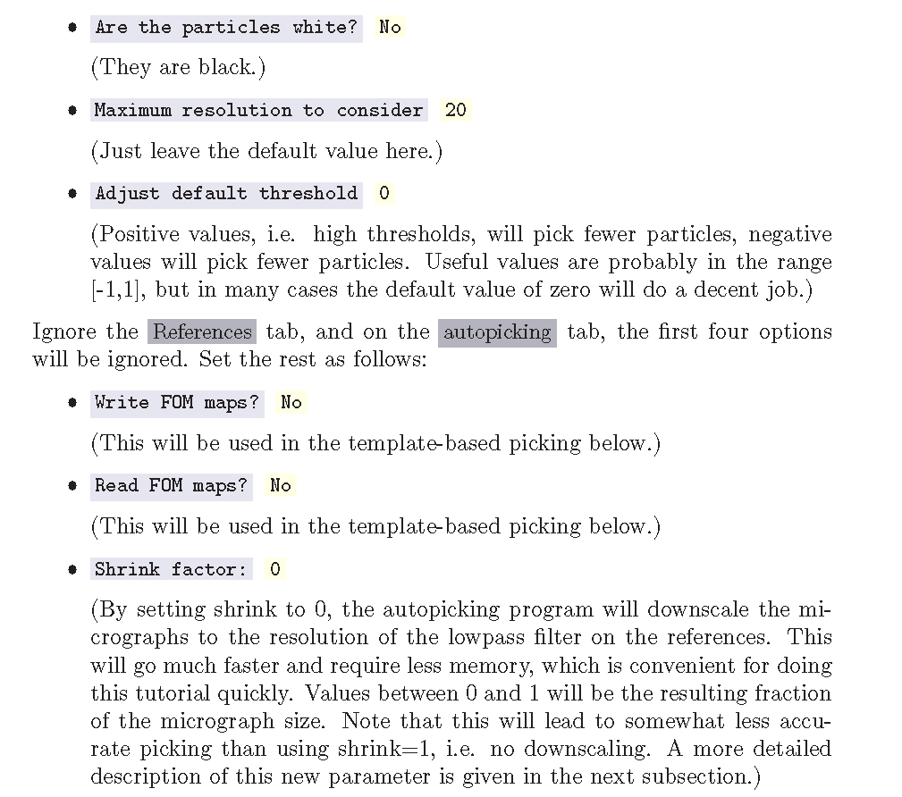
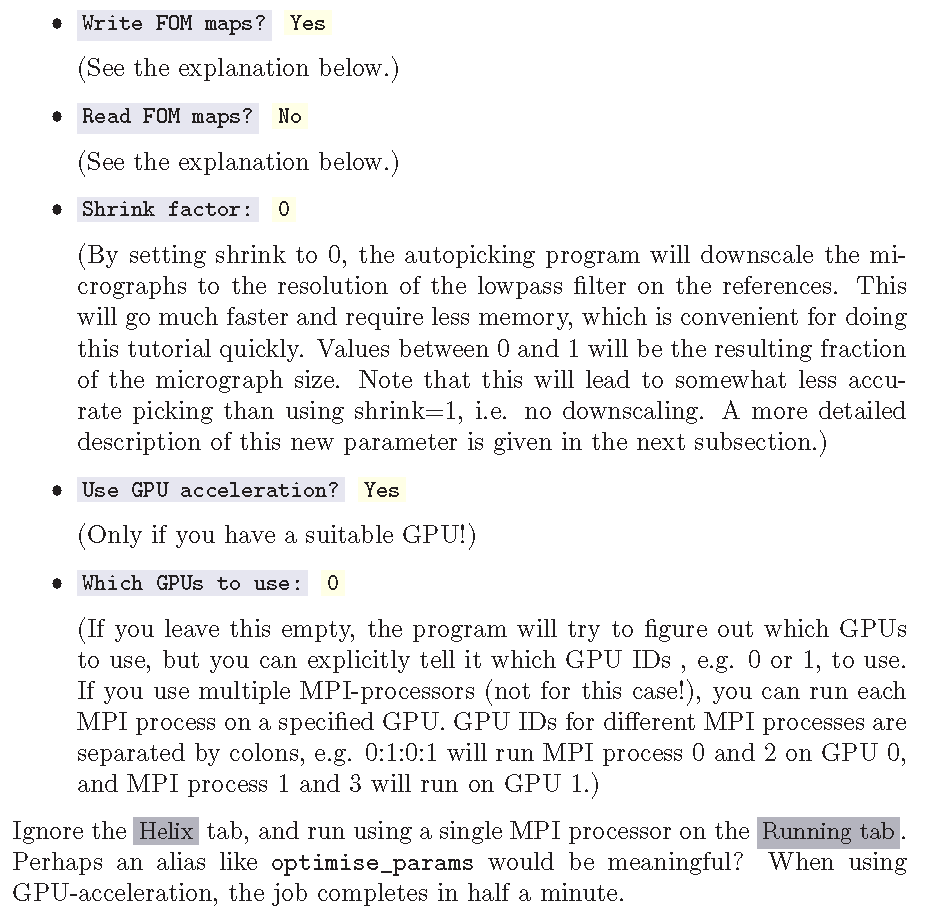
• Write FOM maps? No
• Read FOM maps? Yes
然后点击continue，他就会载入之前保存好的FOM文件而不是重新进行FOM计算，后续新坐标的计算就在几秒内计算完成；后来，我们可以在display出来的图片上右击，选择Reload coordinates 去载入新的coordinates，这个方法能够快速地优化这两个参数。

可以尝试一下修改这三个参数，看看他们是如何改变挑选结果的，当确定了对所有图像自动挑选的参数后，重新选择一个Auto-picking job，然后再I/O tab里换一个输入数据，替换成CTF estimation job中的star file（(CtfFind/job003/micrographs_ctf.star).）；主要参数就按之前那个，不需要改，就在autopicking tab里：
• Picking threshold: 0.0
• Minimum inter-particle distance (A): 100
(Good values are often around 50-70% of the particle diameter.)
• Maximum stddev noise: -1
• Minimum avg noise: -999
• Write FOM maps? No
• Read FOM maps? No
然后running tab里，关于MPI的参数，最大的有效MPI数就是star file中图片的数量；如果使用1个MPI和1个GPU，计算大概耗时1分钟；这个job别名命名为：template_based；

注意的是，当我们continue时，是否read/write FOM maps是一个很重要的区别。如果你write or read FOM map 并且点击continue后，程序将会重新挑选所有输入图像；然而，如果你不read or write FOM map，就比如现在马上要在全部图片中autopick 的第二版Auto Picking job，点击Continue后，只有那些没被自动挑选过的图像会被进行操作，这在迭代计划任务的时候非常有用，比如在显微镜检查过程中实时处理数据。也可以通过13.3查看更多细节；如果是想要在全部图像中用新的参数重新挑选（不是仅在未完成的图像中），然后点击一个新的Auto-picking job——会产生一个新的输出目录。

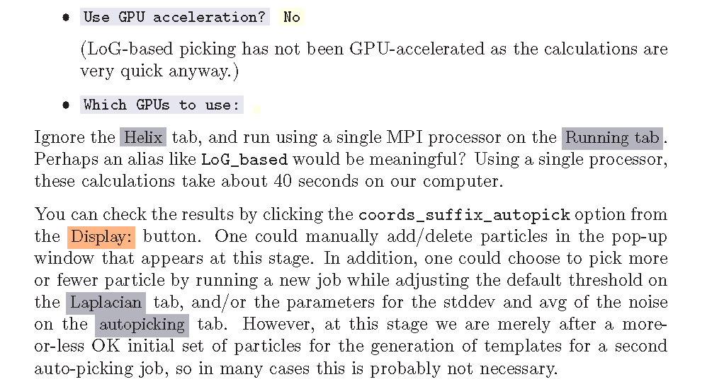
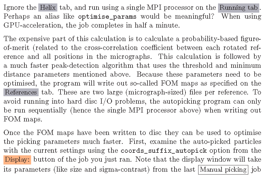
我们可以再通过Display选择cords_suffix_autopick来检查结果，有的人喜欢手动仔细检查所有图像并移除假阳性的颗粒，比如碳边缘和高对比度的合成物就常被错认为是颗粒。

一旦对总体结果满意，为了节省磁盘空间，可能需要删除第一步中编写的FOM-maps，可以使用Job actions中的Gentle clean选项来方便地完成此操作。

当对整个坐标集感到满意，将需要重新运行particle extraction job，保持一切与以前一样，并更改新生成的、自动生成的Input coordinates。;这将生成最初的单粒子数据集，用于下面的进一步细化。也许像template_based这样的别名是有意义的?

1.9 缩放参数（The shrink parameter）

…

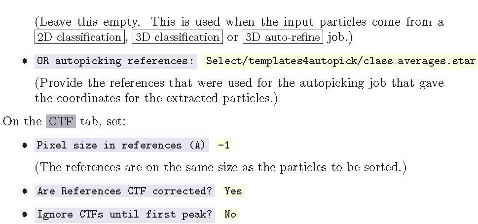
1.10 颗粒排序（particle sorting）

前文extarct出颗粒后，开始对颗粒进行优良排序：

Particle Job：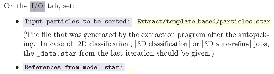


然后可以在out那里看到，particle_sort.star；

接着，Subset selection job，在 OR select from particles.star. 中选择刚刚生成的particle_sort.satr 然后RUN，然后就要选择颗粒了，可以选到一个觉得不大合适的点了，右键select all above，选中前面所有的，然后再右键save，建议将这个subset job命名为after_sorting；

在RELION3.0中可以自动选择sorting颗粒，方法就是在刚才的Subset Selection的job中，现在I/O tab中，OR select from particle中选中刚才的particle_sort.star，其他的注意不要选，再在subsets的tabs中选择参数：
• Select based on metadata vaklues? Yes
• Metadata labal for subset selection rlnParticleSelectZScore
• Minimum metadata value: -9999.
• Maximum metadata value: 0.8
• OR: select on image statistics? No
• OR: split into subsets? No

2 无参考的2D类别平均(Reference-free 2D class averaging)

我们几乎都是使用无参考的2D类别平均来扔掉不好的颗粒。尽管我们经常为了颗粒提取的环节，而在前面的环节中努力只包括好的颗粒（比如对提取的颗粒进行派去，从而进行手动地监督自动挑选的结果），但是还是会存在坏颗粒的情况；因为他们没有平均得很好，经常会有相关的小类别中存在一些很差的2D类别平均。如果能把它们排除掉，就是一个清理我们数据的一个好办法。

2.1 运行JOB

大多数选项和前面生成自动挑选的模板时是一样的，但是在2D classfication job的I/O tab中，设置：
• Input images STAR file: Select/after sorting/particles.star
在Optimisation tab中，设置：
• Number of classes: 100 (because we now have more particles.)

可以命名为after_sorting，然后这个时间要跑的稍长，tutorial说要20min，我们集群倒是不用，就几分钟吧

然后再开始新的Subset selection，select class from model star 中选中咱们刚才生成的model.star，可以命名为class2d_aftersort，然后继续选择、保存；

此时，如果您在自动选择过程中使用了一个较低的阈值，那么您应该非常警惕“Einstein-from-noise”类，这些类看起来像用于选择它们的模板的低分辨率ghost，而高分辨率的噪声可能已经积累在这些模板上，应在选择时避免他们；

选择完全部类别后，保存；

需要注意的是，在2D分类之后，可以(原则上)重新运行sort算法来识别数据中的剩余异常值(尽管我们在实践中不经常这样做)。

2.2 从更多细节上分析结果(Analysing the results in more detail)

tutorial说道：
If you are in a hurry to get through this tutorial, you can skip this sub-section.It contains more detailed information for the interested reader.
然后，我就skip了

2.3 分组(Making groups)

the same as the last step

预处理与2D平均类平均小结：

workflow: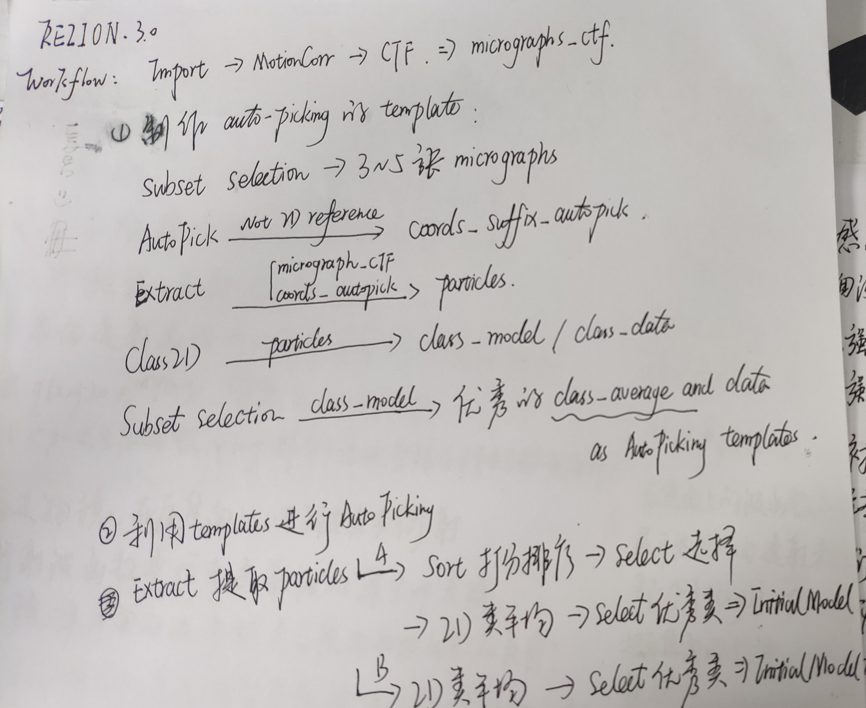

3 生成3维模型（De novo 3D model generation）

RELION使用随机梯度下降法从二维的颗粒图像中，生成初始的三维模型。RELION3.0的方法非常接近cryoSPARC program（附件8）。

如果我们有颗粒各个方向上合理分布的图像且数据量足够大使得2D分类得比较好，这个算法就很可能生成一个低分辨率的模型用于三维重构和后面的三维重构自动调优；

需要注意的是，RELION3.0中，不再需要在2D分类的每个类别中随机选取一部分的颗粒作为子集了，目前的算法非常健壮，使得可以使用全部颗粒作为集合；

3.1 运行作业

选中3D initial model，然后再I/O tab，选中刚刚生成的Select/class2d_aftersort/particles.star，CTF tab则不需要修改，而在optimisation tab页：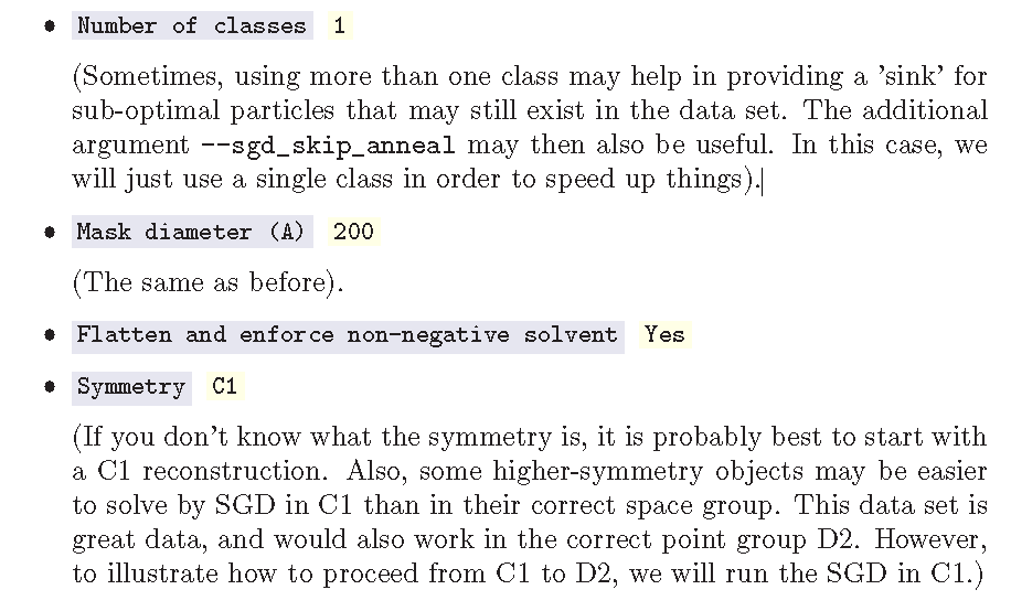

然后SGD tab的话，建议不修改参数，但是为了这个tutorial的加速，我们只是用平常一半的迭代数：
• Number of initial iterations 25
• Number of in-between iterations 100
• Number of final iterations 25

然后在computer的tab里，就根据自己的系统进行优化，我的参数设置：
computer tab: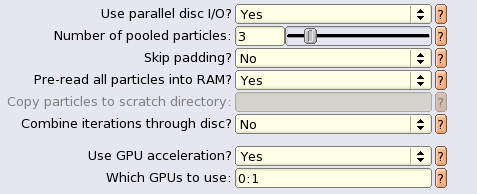

running tab：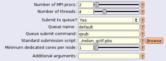

然后是c004节点，ppn=2，我们大概使用了

3.2 分析结果

查看刚才输出的三维图像（(InitialModel/job017/run_it150_class001.mrc)），需要使用chimera软件打开：

首先，登陆baode02：ssh baode02 -Y
然后，输入：chimera 接着打开生成的 InitialModel/job017/run_it150_class001.mrc 那个it后面的数字是迭代到的代数

打开软件后，file -> open 然后选择文件，然后就看到了初始的模型，

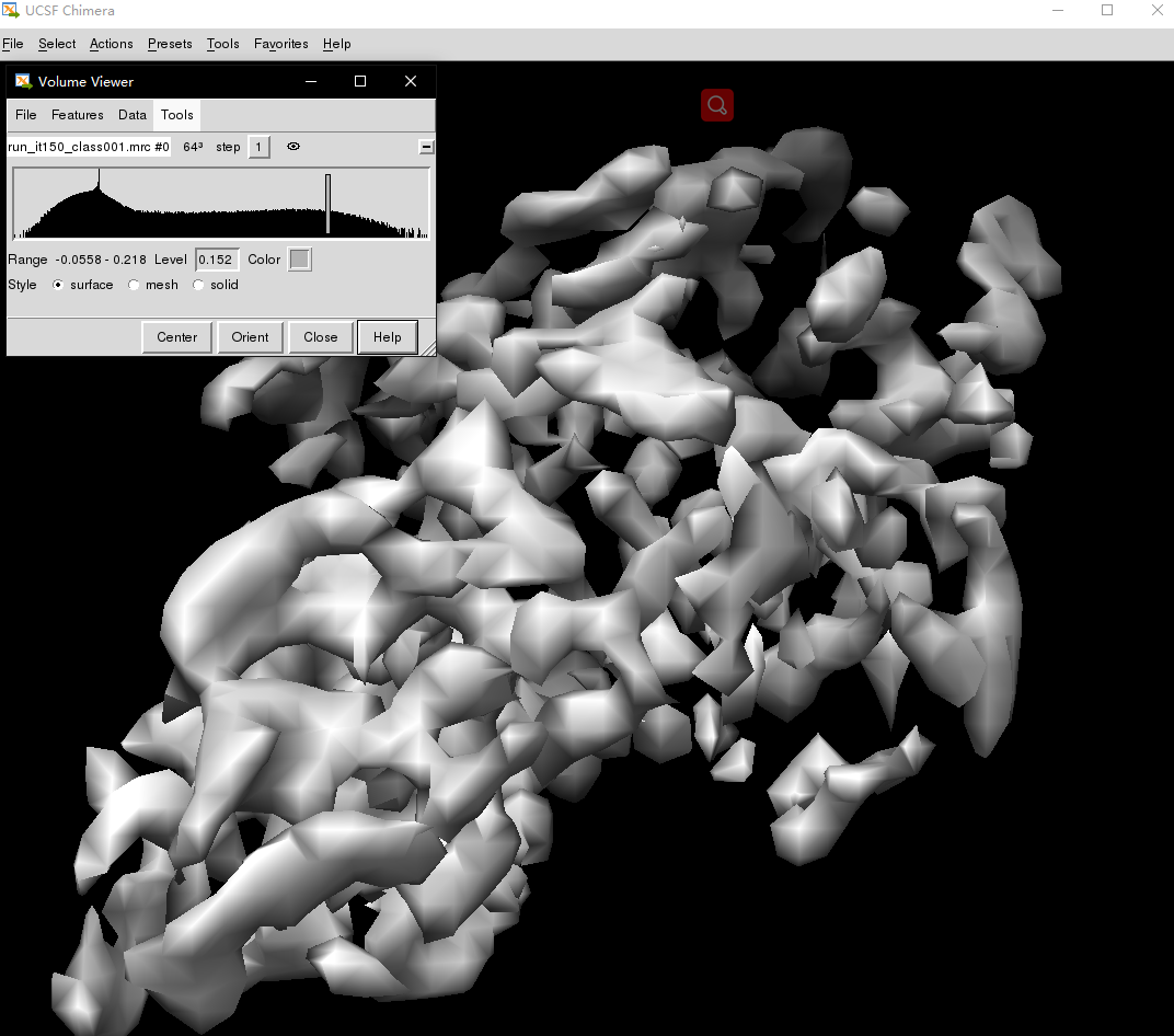
小框里是一个cutoff，通过滑动，可以看到图像的变化，往左是填充，但会变得模糊，左侧高频那个节点会有很散乱的碎片不知道为啥，然后觉得还是一开始打开的默认cutoff下的结构比较清晰、合适，然后可以滚轮缩放，左键拖动角度，右键拖动位置，调整后能够看到和真实颗粒比较相似的结构：

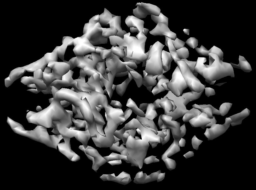
实际的颗粒2D和3D：

如果在这个点上认出了其他的点群对称，按照RELION的惯例，将对称轴和坐标系的主X,Y,Z轴对齐：
Run it as follows from the command line:
relion_align_symmetry —i InitialModel/job017/run_it150_class001.mrc \
—o InitialModel/job017/run_it150_class001_alignD2.mrc —sym D2

And after confirming in UCSF Chimera or relion_display that the symmetry axes in the map are now indeed aligned with the X, Y and Z-axes, we can now impose D2 symmetry using:
relion_image_handler —i InitialModel/job017/run_it150_class001_alignD2.mrc \
—o InitialModel/job017/run_it150_class001_symD2.mrc —sym D2
The output map of the latter command should be similar to the input map.You could check this by:
relion_display —i InitialModel/job017/run_it150_class001_alignD2.mrc &
relion_display —i InitialModel/job017/run_it150_class001_symD2.mrc &

4 无监督的三维分类(Unsupervised 3D classification)

所有的数据集都是不均一的！问题就在于，你有多能忍。RELION的3D多参考调优过程提供了一个有效的无监督3D分类方法；

4.1 运行作业

3D classification：

1. On the I/O tab set:
   • Input images STAR file: Select/class2d aftersort/particles.star
   • Reference map: InitialModel/job017/run it150 class001 symD2.mrc
   (Note that this map does not appear in the Browse button as it is not part of the pipeline. You can either type it’s name into the entry field, or first import the map using the Import jobtype. Also note that, because we wil be running in symmetry C1, we could have also chosen to use the non-symmetric InitialModel/job017/run_it150_class001.mrc. However,already being in the right symmetry setting is more convenient later on.)
   • Reference mask (optional):
   (Leave this empty. This is the place where we for example provided large/small-subunit masks for our focussed ribosome refinements. If left empty, a spherical mask with the particle diameter given on the Optimisation tab will be used. This introduces the least bias into the classification.)

2. On the Reference tab set:
   • Ref. map is on absolute greyscale: Yes
   (Given that this map was reconstructed from this data set, it is already on the correct greyscale. Any map that is not reconstructed from the same data in relion should probably be considered as not being on the correct greyscale.)
   • Initial low-pass filter (A): 50
   (One should NOT use high-resolution starting models as they may introduce bias into the refinement process. As also explained in [12], one should filter the initial map as much as one can. For ribosome we often use 70°A,
   for smaller particles we typically use values of 40-60°A.)
   • Symmetry: C1
   (Although we know that this sample has D2 symmetry, it is often a good idea to perform an initial classification without any symmetry,so bad particles, which are not symmetry, can get separated from proper ones, and the symmetry can be verified in the reconstructed maps.)

3. On the CTF tab set:
   • Do CTF correction? Yes
   • Has reference been CTF-corrected? Yes
   (As this model was made using CTF-correction in the SGD.)
   • Have data been phase flipped? No
   • Ignore CTFs until first peak? No
   (Only use this option if you also did so in the 2D classification job that you used to create the references.)

4. On the Optimisation tab set:

   • Number of classes: 4
   (Using more classes will divide the data set into more subsets, potentially
   describing more variability. The computational costs scales linearly with
   the number of classes, both in terms of CPU time and required computer
   memory.)
   • Number of iterations: 25
   (We typically do not change this.)
   • Regularisation parameter T: 4
   For the exact definition of T, please refer to [13]. For cryo-EM 2D classification we typically use values of T=1-2, and for 3D classification values of 2-4. For negative stain sometimes slightly lower values are better. In general, if your class averages appear noisy, then lower T; if your class averages remain too-low resolution, then increase T. The main thing isto be aware of overfitting high-resolution noise. We happened to use a value of 2 in our pre-calculated results. Probably a value of 4 would have worked equally well…
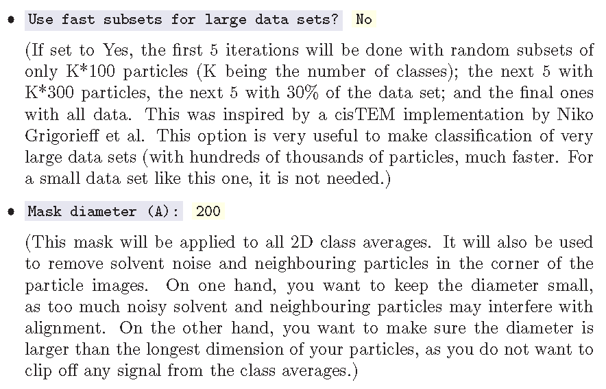
   • Mask diameter (A): 200
   (Just use the same value as we did before in the 2D classification job-type.)
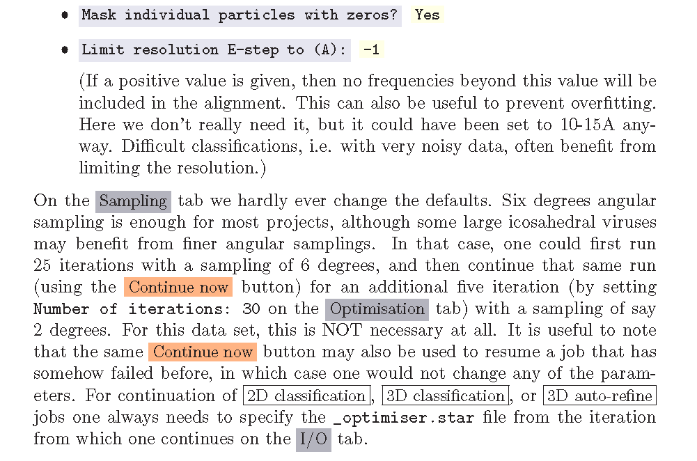
   • Mask individual particles with zeros? Yes
   • Limit resolution E-step to (A): -1
   (If a positive value is given, then no frequencies beyond this value will be included in the alignment. This can also be useful to prevent overfitting.Here we don’t really need it, but it could have been set to 10-15A anyway.)

   而sampling tab一般不需要修改参数，