不平衡采样
各种不平衡采样,欠采样、过采样、SMOTE均衡采样、组合采样、集成采样、模型选择和特征选择
Various Sampling methods, Under Sampling, Over Sampling, SMOTE balanced sampling, Combination Sampling, Ensemble Sampling, Model Selection, and Feature Selection
参考:
欠采样
随机欠采样
class imblearn.under_sampling.RandomUnderSampler(*, sampling_strategy=’auto’, random_state=None, replacement=False
下面的example是最简单的欠采样,当然还有很多种欠采样,可以参考:Under-sampling methods,
1 | from collections import Counter |
聚类采样
基本用法
class imblearn.under_sampling.ClusterCentroids(*, sampling_strategy=’auto’, random_state=None, estimator=None, voting=’auto’, n_jobs=’deprecated’)[source]
1 | from imblearn.under_sampling import ClusterCentroids |
主要参数:sampling_strategy=’auto’, random_state=None, estimator=None, voting=’auto’
sampling_strategy是比例:
sampling_strategyfloat, str, dict, callable, default=’auto’
Sampling information to sample the data set.
- When
float, it corresponds to the desired ratio of the number of samples in the minority class over the number of samples in the majority class after resampling. Therefore, the ratio is expressed as where
where  is the number of samples in the minority class and
  is the number of samples in the majority class after resampling.
estimatorestimator object, default=None
Pass a KMeans estimator. By default, it will be a default KMeans estimator.
voting{“hard”, “soft”, “auto”}, default=’auto’
Voting strategy to generate the new samples:
- If
'hard', the nearest-neighbors of the centroids found using the clustering algorithm will be used. - If
'soft', the centroids found by the clustering algorithm will be used. - If
'auto', if the input is sparse, it will default on'hard'otherwise,'soft'will be used.
NearMiss
class imblearn.under_sampling.NearMiss(*, sampling_strategy=’auto’, version=1, n_neighbors=3, n_neighbors_ver3=3, n_jobs=None)
基本用法
1 | from imblearn.under_sampling import NearMiss |
关键参数:version=1,n_neighbors=3, n_neighbors_ver3=3
version: int, default=1
Version of the NearMiss to use. Possible values are 1, 2 or 3.
n_neighbors:int or estimator object, default=3
If int, size of the neighbourhood to consider to compute the average distance to the minority point samples. If object, an estimator that inherits from KNeighborsMixin that will be used to find the k_neighbors. By default, it will be a 3-NN.
n_neighbors_ver3: int or estimator object, default=3
If int, NearMiss-3 algorithm start by a phase of re-sampling. This parameter correspond to the number of neighbours selected create the subset in which the selection will be performed. If object, an estimator that inherits from KNeighborsMixin that will be used to find the k_neighbors. By default, it will be a 3-NN.
其中,关于NearMiss的版本,官方介绍,简单解释
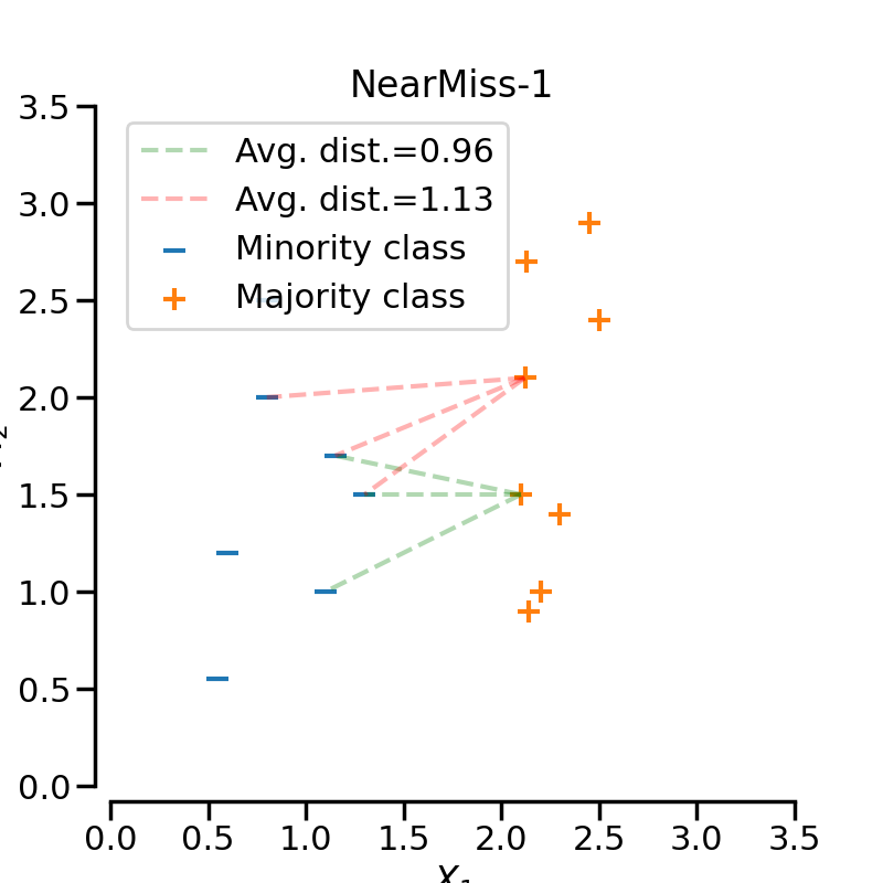
NearMiss-1
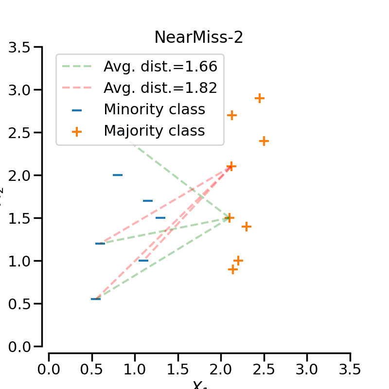
选择到最近的三个少数类样本平均距离最小的那些多数类样本NearMiss-2
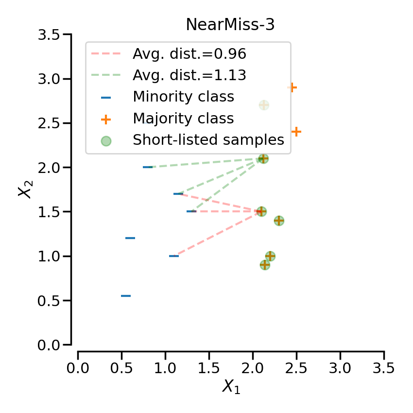
选择到最远的三个少数类样本平均距离最小的那些多数类样本NearMiss-3
为每个少数类样本选择给定数目的最近多数类样本,目的是保证每个少数类样本都被一些多数类样本包围
Note:实验结果表明一般NearMiss-2 方法的不均衡分类性能最优
TomekLinks
class imblearn.under_sampling.TomekLinks(*, sampling_strategy=’auto’, n_jobs=None)
基本用法
1 | tl = TomekLinks() |
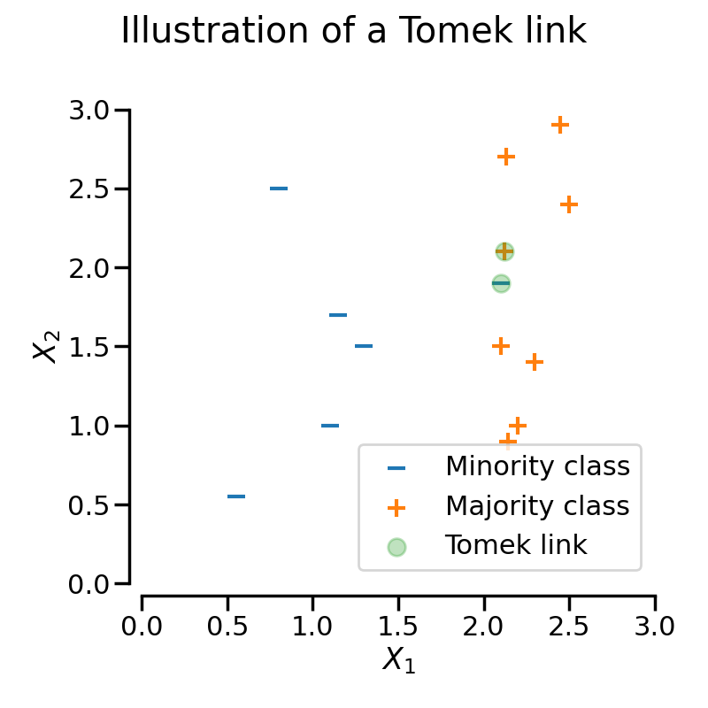
TomekLinks detects the so-called Tomek’s links [Tom76b]. A Tomek’s link between two samples of different class  and
and  is defined such that for any sample
  :
:

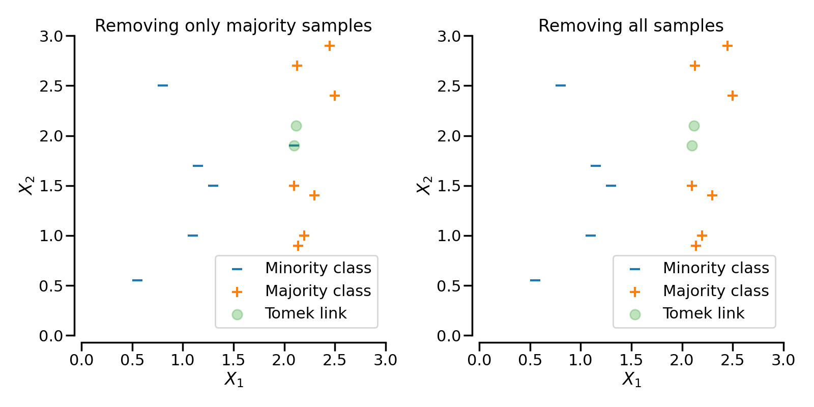
where  is the distance between the two samples. In some other words, a Tomek’s link exist if the two samples are the nearest neighbors of each other. In the figure below, a Tomek’s link is illustrated by highlighting the samples of interest in green.is the distance between the two samples. In some other words, a Tomek’s link exist if the two samples are the nearest neighbors of each other. In the figure below, a Tomek’s link is illustrated by highlighting the samples of interest in green.
关键参数:
sampling_strategy: str, list or callable
Sampling information to sample the data set.
When
str, specify the class targeted by the resampling. Note the the number of samples will not be equal in each. Possible choices are:'majority': resample only the majority class;'not minority': resample all classes but the minority class;'not majority': resample all classes but the majority class;'all': resample all classes;'auto': equivalent to'not minority'.When
list, the list contains the classes targeted by the resampling.When callable, function taking
yand returns adict. The keys correspond to the targeted classes. The values correspond to the desired number of samples for each class.
The parameter sampling_strategy control which sample of the link will be removed. For instance, the default (i.e., sampling_strategy='auto') will remove the sample from the majority class. Both samples from the majority and minority class can be removed by setting sampling_strategy to 'all'. The figure illustrates this behaviour.
EditedNearestNeighbours
因为随机欠抽样方法未考虑样本的分布情况,采样具有很大的随机性,可能会删除重要的多数类样本信息。针对以上的不足,Wilson 等人提出了一种最近邻规则(edited nearest neighbor: ENN)。
基本思想:删除那些类别与其最近的三个近邻样本中的两个或两个以上的样本类别不同的样本
缺点:因为大多数的多数类样本的样本附近都是多数类,所以该方法所能删除的多数类样本十分有限。
基本用法
1 | from imblearn.under_sampling import EditedNearestNeighbours |
关键参数:
*n_neighbors=3*
kind_sel{‘all’, ‘mode’}, default=’all’
Strategy to use in order to exclude samples.
- If
'all', all neighbours will have to agree with the samples of interest to not be excluded. / 所有的邻居都要同类 - If
'mode', the majority vote of the neighbours will be used in order to exclude a sample. / 邻居中同类占多数
The strategy "all" will be less conservative than 'mode'. Thus, more samples will be removed when kind_sel="all" generally.
RepeatedEditedNearestNeighbours
RepeatedEditedNearestNeighbours extends EditedNearestNeighbours by repeating the algorithm multiple times [Tom76a]. Generally, repeating the algorithm will delete more data:
关键参数: max_iter=100
1 | from imblearn.under_sampling import RepeatedEditedNearestNeighbours |
ALLKNN
This method will apply ENN several time and will vary the number of nearest neighbours.
AllKNN differs from the previous RepeatedEditedNearestNeighbours since the number of neighbors of the internal nearest neighbors algorithm is increased at each iteration [Tom76a]
CondensedNearestNeighbour
使用1近邻的方法来进行迭代, 来判断一个样本是应该保留还是剔除, 具体的实现步骤如下:
- 集合C: 所有的少数类样本;
- 选择一个多数类样本(需要下采样)加入集合C, 其他的这类样本放入集合S;
- 使用集合S训练一个1-NN的分类器, 对集合S中的样本进行分类;
- 将集合S中错分的样本加入集合C;
- 重复上述过程, 直到没有样本再加入到集合C.
NeighbourhoodCleaningRule
基本用法
1 | from collections import Counter |
InstanceHardnessThreshold
基本用法:
InstanceHardnessThreshold is a specific algorithm in which a classifier is trained on the data and the samples with lower probabilities are removed [SMGC14]. The class can be used as:
1 | from sklearn.linear_model import LogisticRegression |
This class has 2 important parameters. estimator will accept any scikit-learn classifier which has a method predict_proba. The classifier training is performed using a cross-validation and the parameter cv can set the number of folds to use.
关键参数:
estimator: estimator object, default=None
Classifier to be used to estimate instance hardness of the samples. By default a RandomForestClassifier will be used. If str, the choices using a string are the following: 'knn', 'decision-tree', 'random-forest', 'adaboost', 'gradient-boosting' and 'linear-svm'. If object, an estimator inherited from ClassifierMixin and having an attribute predict_proba.
cv: int, default=5
Number of folds to be used when estimating samples’ instance hardness.
难例阈值的确定
过采样
class imblearn.over_sampling.RandomOverSampler(*, sampling_strategy=’auto’, random_state=None, shrinkage=None)[source]
下面的example是最简单的过采样,当然还有很多种欠采样,可以参考:Under-sampling methods,
1 | from imblearn.over_sampling import RandomOverSampler |
SMOTE
官方文档: SMOTE
Naive SMOTE
class imblearn.over_sampling.SMOTE(*, sampling_strategy=’auto’, random_state=None, k_neighbors=5, n_jobs=None)
SMOTE(Synthetic Minority Oversampling Technique)合成少数类过采样技术,是在随机采样的基础上改进的一种过采样算法。
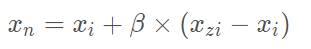
首先,从少数类样本中选取一个样本xi。其次,按采样倍率N,从xi的K近邻中随机选择N个样本xzi。最后,依次在xzi和xi之间随机合成新样本,合成公式如下:
SMOTE实现简单,但其弊端也很明显,由于SMOTE对所有少数类样本一视同仁,并未考虑近邻样本的类别信息,往往出现样本混叠现象,导致分类效果不佳。
1 | from collections import Counter |
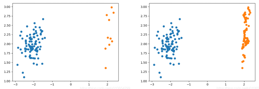
SMOTE采样前后对比
Borderline SMOTE
论文地址:http://xueshu.baidu.com/usercenter/paper/show?paperid=f95a4bd0843c4c6389cc878bc1d525a2&site=xueshu_se
Borderline SMOTE是在SMOTE基础上改进的过采样算法,该算法仅使用边界上的少数类样本来合成新样本,从而改善样本的类别分布。
Borderline SMOTE采样过程是将少数类样本分为3类,分别为Safe、Danger和Noise,具体说明如下。最后,仅对表为Danger的少数类样本过采样。
Safe,样本周围一半以上均为少数类样本,如图中点A
Danger:样本周围一半以上均为多数类样本,视为在边界上的样本,如图中点B
Noise:样本周围均为多数类样本,视为噪音,如图中点C

Borderline-SMOTE又可分为Borderline-SMOTE1和Borderline-SMOTE2,Borderline-SMOTE1在对Danger点生成新样本时,在K近邻随机选择少数类样本(与SMOTE相同),Borderline-SMOTE2则是在k近邻中的任意一个样本(不关注样本类别)
Borderline-SMOTE Python使用
class imblearn.over_sampling.BorderlineSMOTE(*, sampling_strategy=’auto’, random_state=None, k_neighbors=5, n_jobs=None, m_neighbors=10, kind=’borderline-1’) [source]
1 | from collections import Counter |
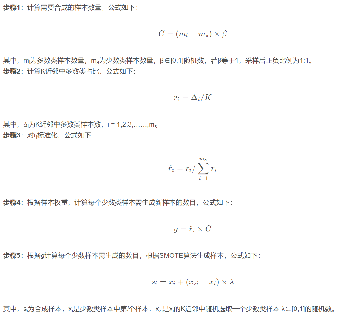
ADASYN
论文地址:http://xueshu.baidu.com/usercenter/paper/show?paperid=13cbcaf6a33e0e3df06c0c0c421209d0&site=xueshu_se
ADASYN (adaptive synthetic sampling)自适应合成抽样,与Borderline SMOTE相似,对不同的少数类样本赋予不同的权重,从而生成不同数量的样本。具体流程如下:
ADASYN Python使用
1 | from collections import Counter |
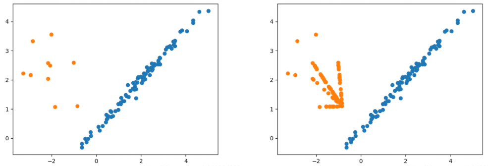
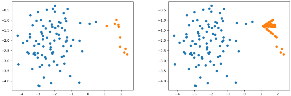
ADASYN 采样前后对比
SMOTENC
class imblearn.over_sampling.SMOTENC(categorical_features, *, sampling_strategy=’auto’, random_state=None, k_neighbors=5, n_jobs=None)
因为SMOTE算法和ADASY算法在上采样的时候用到了距离,因此当x xx为异构数据,即含有离散变量(例如0代表男,1代表女),此时无法直接对离散变量使用欧氏距离。因此有了变体SMOTENC,其在处理离散数据时,采用K近邻样本中出现频率最高的离散数据作为新的样本的值。但是要提前告知离散数据出现的维度位置。
1 | from imblearn.over_sampling import BorderlineSMOTE |
此外,还有专门针对全部都是categorical features的SMOTEN:Over-sample using the SMOTE variant specifically for categorical features only.
SVMSMOTE
class imblearn.over_sampling.SVMSMOTE(*, sampling_strategy=’auto’, random_state=None, k_neighbors=5, n_jobs=None, m_neighbors=10, svm_estimator=None, out_step=0.5)
使用SVM分类器找到支持向量,在生成的时候会考虑它们. SVM的C参数决定了选择支持向量的多少
Variant of SMOTE algorithm which use an SVM algorithm to detect sample to use for generating new synthetic samples as proposed in [2].
Read more in the User Guide.
KMeansSMOTE
class imblearn.over_sampling.KMeansSMOTE(*, sampling_strategy=’auto’, random_state=None, k_neighbors=2, n_jobs=None, kmeans_estimator=None, cluster_balance_threshold=’auto’, density_exponent=’auto’)
Apply a KMeans clustering before to over-sample using SMOTE.
This is an implementation of the algorithm described in [1].
Read more in the User Guide.
Combination of over- and under-sampling
We previously presented SMOTE and showed that this method can generate noisy samples by interpolating new points between marginal outliers and inliers. This issue can be solved by cleaning the space resulting from over-sampling.
In this regard, Tomek’s link and edited nearest-neighbours are the two cleaning methods that have been added to the pipeline after applying SMOTE over-sampling to obtain a cleaner space. The two ready-to use classes imbalanced-learn implements for combining over- and undersampling methods are: (i) SMOTETomek [BPM04] and (ii) SMOTEENN [BBM03].
基本用法
1 | from collections import Counter |
关键参数:
smote: sampler object, default=None
The SMOTE object to use. If not given, a SMOTE object with default parameters will be given.
enn: sampler object, default=None
The EditedNearestNeighbours object to use. If not given, a EditedNearestNeighbours object with sampling strategy=’all’ will be given.
tomek: sampler object, default=None
The TomekLinks object to use. If not given, a TomekLinks object with sampling strategy=’all’ will be given.
Ensemble resampling
BalancedBaggingClassifier
In ensemble classifiers, bagging methods build several estimators on different randomly selected subset of data. In scikit-learn, this classifier is named BaggingClassifier. However, this classifier does not allow to balance each subset of data. Therefore, when training on imbalanced data set, this classifier will favor the majority classes:
1 | from sklearn.datasets import make_classification |
In BalancedBaggingClassifier, each bootstrap sample will be further resampled to achieve the sampling_strategy desired. Therefore, BalancedBaggingClassifier takes the same parameters than the scikit-learn BaggingClassifier. In addition, the sampling is controlled by the parameter sampler or the two parameters sampling_strategy and replacement, if one wants to use the RandomUnderSampler:
1 | from imblearn.ensemble import BalancedBaggingClassifier |
Changing the sampler will give rise to different known implementation [MO97], [HKT09], [WY09]. You can refer to the following example shows in practice these different methods: Bagging classifiers using sampler
BalancedRandomForestClassifier
BalancedRandomForestClassifier is another ensemble method in which each tree of the forest will be provided a balanced bootstrap sample [CLB+04]. This class provides all functionality of the RandomForestClassifier:
1 | > from imblearn.ensemble import BalancedRandomForestClassifier |
RUSBoostClassifier
Several methods taking advantage of boosting have been designed.
RUSBoostClassifier randomly under-sample the dataset before to perform a boosting iteration [SKVHN09]:
1 | from imblearn.ensemble import RUSBoostClassifier |
Bagging - AdaBoostClassifier
A specific method which uses AdaBoostClassifier as learners in the bagging classifier is called “EasyEnsemble”.
The EasyEnsembleClassifier allows to bag AdaBoost learners which are trained on balanced bootstrap samples [LWZ08]. Similarly to the BalancedBaggingClassifier API, one can construct the ensemble as:
1 | from imblearn.ensemble import EasyEnsembleClassifier |
Model selection
偷懒一下…
Feature selection
偷懒两下…